Tip
All input files can be downloaded: Files.
Tip
For more information of this section, please refer to these pages:
MSDFT (4): Charge Transfer Excitations
This tutorial will lead you step by step to study excited states using Multi-State Density Functional Theory (MSDFT).
MSDFT is a powerful method for studying excited states. It optimizes excited states using TSO-DFT method, so it is free of orbital relaxation problem like in TDDFT. In this section, you will see that MSDFT can give much more reasonable results than TDDFT for excited states.
In TSO-DFT (1): Excited States, we have introduced how to use TSO-DFT to study excited states. In MSDFT (1): All Types of Excited States, we have introduced how to use MSDFT to study excitations generally. In MSDFT (2): Core Ionizations and Excitations, we have introduced how to use MSDFT to study core excitations. In MSDFT (3): Double Excitations, we have introduced how to use MSDFT to study double excitations. In this tutorial, we will introduce how to use MSDFT to study charge transfer excitations. We strongly recommend you to read these tutorials before reading this tutorial.
Actually, MSDFT can be considered as TSO+NOSI. MSDFT is a framework that automaitcally performs TSO-DFT and NOSI for required excited states. Of course, you can also perform TSO-DFT and NOSI separately for special purposes.
Example: Charge Transfer Excitations of [TCNE][CH3OCH=CH2]
In this example, we will calculate the charge transfer excitations of the complex [TCNE][CH3OCH=CH2], whiere TCNE is tetracyanoethylene. First, let us calculate its ground state to see its orbitals.
 1basis
 2    cc-pVDZ # In product studies, you should use cc-pVTZ at least.
 3end
 4
 5scf
 6    charge  0
 7    spin2p1 1
 8    type    U
 9end
10
11mol
12           C      -0.198382    0.676975    0.839378
13           C      -1.315863    0.038931    0.405996
14           C      -2.225365    0.670286   -0.508436
15           N      -2.959552    1.174482   -1.247154
16           C      -1.634267   -1.289698    0.850726
17           N      -1.901673   -2.352749    1.221105
18           C       0.723624    0.024005    1.725081
19           N       1.483401   -0.507944    2.417545
20           C       0.131547    2.005023    0.406927
21           N       0.406859    3.079229    0.077027
22           C      -0.018608   -1.360064   -2.097094
23           C       1.086004   -1.277514   -1.352322
24           H      -0.458263   -2.333443   -2.305731
25           H      -0.471114   -0.462748   -2.522620
26           H       1.590935   -2.157076   -0.934177
27           O       1.621801   -0.078506   -1.011442
28           C       2.981195   -0.123945   -0.597217
29           H       3.629890   -0.409943   -1.438672
30           H       3.239414    0.887438   -0.263120
31           H       3.112168   -0.831294    0.237956
32end
33
34task
35    energy b3lyp
36end
After calculation, we can visualize msdft-4-gs.mwfn using Qbics-MolStar. First drag msdft-4-gs.mwfn into explorer, and it will be automatically loaded. Right-click msdft-4-gs.mwfn and select View Molecular Orbitals, click orbital 48, 49, and 50:


Obviously, MO48 is the HOMO mainly localized on CH3OCH=CH2, and MO49 and MO50 are the unoccupied π* and σ* orbitals mainly localized on TCNE, so excitation 48(HOMO) → 49 (LUMO) and 48(HOMO) → 50 (LUMO+1) are both close to but not perfect charge transfer. It seems that MO50 is more localized on TCNE but MO49 still has a few components on CH3OCH=CH2. We will use MSDFT to calculate these 2 excitations:
 1basis
 2    cc-pVDZ # In product studies, you should use cc-pVTZ at least.
 3end
 4
 5scf
 6    charge  0
 7    spin2p1 1
 8    type    U
 9end
10
11mol
12           C      -0.198382    0.676975    0.839378
13           C      -1.315863    0.038931    0.405996
14           C      -2.225365    0.670286   -0.508436
15           N      -2.959552    1.174482   -1.247154
16           C      -1.634267   -1.289698    0.850726
17           N      -1.901673   -2.352749    1.221105
18           C       0.723624    0.024005    1.725081
19           N       1.483401   -0.507944    2.417545
20           C       0.131547    2.005023    0.406927
21           N       0.406859    3.079229    0.077027
22           C      -0.018608   -1.360064   -2.097094
23           C       1.086004   -1.277514   -1.352322
24           H      -0.458263   -2.333443   -2.305731
25           H      -0.471114   -0.462748   -2.522620
26           H       1.590935   -2.157076   -0.934177
27           O       1.621801   -0.078506   -1.011442
28           C       2.981195   -0.123945   -0.597217
29           H       3.629890   -0.409943   -1.438672
30           H       3.239414    0.887438   -0.263120
31           H       3.112168   -0.831294    0.237956
32end
33
34msdft
35    single_ex 48 : 49 50
36end
37
38task
39    msdft b3lyp
40end
msdft...endindicates the MSDFT calculation. Here,single_ex 48 : 49 50means we want to study the single excitation from orbitals 48 to orbitals 49 and 50. Explicitly, we want to study the following single excitations:48 → 49
48 → 50
In the output file msdft-4-ct.out, we can find the following information:
 1---- NOSI Results ----
 2======================
 3   State   NOSI Energies  Excited Energy       Osc. Str.        DX        DY        DZ
 4               (Hartree)            (eV)                    (a.u.)    (a.u.)    (a.u.)
 5       0   -640.67704670      0.00000000      0.00000000  -1.24736   0.66912   0.44355
 6       1   -640.56771187      2.97500080      0.00000000  -0.00000  -0.00000   0.00000
 7       2   -640.55543283      3.30911339      0.17632767  -1.18048   0.77057   1.54122
 8       3   -640.54664537      3.54822018      0.00000000   0.00000  -0.00000  -0.00000
 9       4   -640.42108402      6.96474459      0.55299075   2.03421   0.55834   1.43209
10
11---- NOSI State Identification (Coefficients) ----
12==================================================
13State |0> = -0.999 |msdft-4-ct-gs.mwfn>
14State |1> = +0.710 |msdft-4-ct-48-to-49-se.mwfn> -0.710 |spin_flip_msdft-4-ct-48-to-49-se.mwfn>
15State |2> = -0.700 |msdft-4-ct-48-to-49-se.mwfn> -0.700 |spin_flip_msdft-4-ct-48-to-49-se.mwfn>
16State |3> = -0.708 |msdft-4-ct-48-to-50-se.mwfn> +0.708 |spin_flip_msdft-4-ct-48-to-50-se.mwfn>
17State |4> = -0.707 |msdft-4-ct-48-to-50-se.mwfn> -0.707 |spin_flip_msdft-4-ct-48-to-50-se.mwfn>
State 2 and 4 are singlet charge transfer excitations.
Example: Distance-Dependence of Charge Transfer Excitations
Theoretical analysis reveals that the charge transfer excitation energies \(\omega\) and the distance between the acceptor and donor \(d\) has such a relationship:
However, conventional TDDFT cannot repoduce this relationship because TDDFT has systematic error for charge transfer excitations! Let’s see if MSDFT can reproduce this relationship for the above example.
Generate Structures
To study the distance dependence, we will generate a series of [TCNE][CH3OCH=CH2] structures that the donor and acceptor departs. First, we save the structure in msdft-4-gs.inp in an XYZ file called r0.xyz:
 120
 2d = 3.21 Angstrom
 3C      -0.198382    0.676975    0.839378
 4C      -1.315863    0.038931    0.405996
 5C      -2.225365    0.670286   -0.508436
 6N      -2.959552    1.174482   -1.247154
 7C      -1.634267   -1.289698    0.850726
 8N      -1.901673   -2.352749    1.221105
 9C       0.723624    0.024005    1.725081
10N       1.483401   -0.507944    2.417545
11C       0.131547    2.005023    0.406927
12N       0.406859    3.079229    0.077027
13C      -0.018608   -1.360064   -2.097094
14C       1.086004   -1.277514   -1.352322
15H      -0.458263   -2.333443   -2.305731
16H      -0.471114   -0.462748   -2.522620
17H       1.590935   -2.157076   -0.934177
18O       1.621801   -0.078506   -1.011442
19C       2.981195   -0.123945   -0.597217
20H       3.629890   -0.409943   -1.438672
21H       3.239414    0.887438   -0.263120
22H       3.112168   -0.831294    0.237956
Now, we write a python script to generate a series of structures:
 1#!/usr/bin/python3
 2
 3def read_xyz(path):
 4    with open(path, 'r') as f:
 5        lines = f.readlines()
 6    natoms = int(lines[0].strip())
 7    title = lines[1].rstrip("\n")
 8    coords = [line.rstrip("\n") for line in lines[2:]]
 9    if len(coords) != natoms:
10        raise ValueError("The number of atoms is inconsistent with the first line")
11    return natoms, title, coords
12
13def write_xyz(path, natoms, title, coords):
14    with open(path, 'w') as f:
15        f.write(f"{natoms}\n")
16        f.write(f"{title}\n")
17        for line in coords:
18            f.write(f"{line}\n")
19
20def translate_atoms(coords, vector, start_idx, end_idx):
21    dx, dy, dz = vector
22    for i in range(start_idx, end_idx + 1):
23        if i >= len(coords):
24            break
25        parts = coords[i].split()
26        if len(parts) < 4:
27            raise ValueError(f"Line {i+3} format error: {coords[i]}")
28        sym, x, y, z = parts[0], float(parts[1]), float(parts[2]), float(parts[3])
29        x += dx
30        y += dy
31        z += dz
32        coords[i] = f"{sym:>2s} {x:15.8f} {y:15.8f} {z:15.8f}"
33    return coords
34
35if __name__ == "__main__":
36    dx = (-0.198382)-1.086004
37    dy = (0.676975)-(-1.277514)
38    dz = (0.839378)-(-1.352322)
39    r = (dx*dx+dy*dy+dz*dz)**0.5
40    ex = dx/r
41    ey = dy/r
42    ez = dz/r
43    in_file = "r0.xyz"
44    for i in range(1,9):
45        natoms, title, coords = read_xyz(in_file)
46        dr = 0.5*i
47        d = 3.21+dr
48        vector = (ex*dr, ey*dr, ez*dr)
49        coords = translate_atoms(coords, vector, start_idx=0, end_idx=9)
50        out_file = f"r{i:d}.xyz"
51        title = f"d = {d:.2f} Angstrom"
52        write_xyz(out_file, natoms, title, coords)
53        print(f"Write {out_file}.")
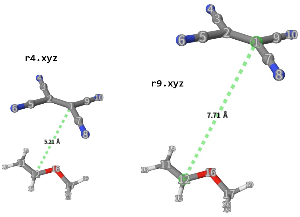
Run this python script by ./generate_structure.py and we will generate 14 structures, with TCNE moving along axis atom 1-12 by 0.5 Angstorm every time. See below:
Calculate Energies
Now, prepare the input file:
 1basis
 2    cc-pVDZ # In product studies, you should use cc-pVTZ at least.
 3end
 4
 5scf
 6    charge  0
 7    spin2p1 1
 8    type    U
 9end
10
11mol
12    r0.xyz
13end
14
15msdft
16    single_ex 48 : 49 50
17end
18
19task
20    msdft b3lyp
21end
Now, we write a shell script to run the 15 calculations by replacing r0.xyz to r1.xyz, etc.:
1inp=msdft-4-rd.inp
2for i in {0..9}; do
3    sed "s/r0\.xyz/r${i}.xyz/g" "$inp" > "msdft-4-r${i}.inp"
4    # Replace qbics-linux-cpu to the suitable one for your system
5    qbics-linux-cpu "msdft-4-r${i}.inp" -n 24 > "msdft-4-r${i}.out"
6done
When all calculations are completed, we can extract excitation energies to energies.txt:
1out="energies.txt"
2echo "Distance E1 E2" > ${out}
3for i in {0..9}; do
4    d=$(echo "3.21 + $i * 0.5" | bc -l)
5    read -r e1 e2 < <(awk 'NR==3{printf "%s ",$3} NR==5{printf "%s",$3}' "msdft-4-r${i}-spectrum.txt")
6    echo "$d $e1 $e2" >> ${out}
7done
Fit and Plot Data
Now, we write a python script to read the distances and excitation energies, fit the energies with respect to \(\omega=A+\frac{B}{d}\), and plot them:
 1#!/usr/bin/python3
 2
 3import matplotlib.pyplot as plt
 4import numpy as np
 5import matplotlib.gridspec as gridspec
 6from scipy.stats import linregress
 7
 8# Fit data.
 9def fit(a, b):
10    res = linregress(a, b)
11    return a*res.slope+res.intercept, res
12
13# Get data.
14fn   = "energies.txt"
15data = np.loadtxt(fn, skiprows = 1).transpose()
16d    = data[0]
17e1   = data[1]
18e2   = data[2]
19idx1 = 4
20idx2 = 2
21d1_fit = d[idx1:]
22d2_fit = d[idx2:]
23e1_fit, res1 = fit(1/d1_fit, e1[idx1:])
24e2_fit, res2 = fit(1/d2_fit, e2[idx2:])
25
26# Draw figures.
27plt.subplot(1, 2, 1)
28plt.plot(d, e1, "ro", label="Excitation: 48->49")
29plt.plot(d1_fit, e1_fit, "r-", label="Fit")
30plt.text(4, 3.35, f"$\omega = {res1.intercept:.3f}{res1.slope:.3f}/d$", fontsize=12, color='red')
31plt.text(4, 3.33, f"$R^2$ = {res1.rvalue**2:.3f}", fontsize=12, color='red')
32plt.xlabel("$d$ (Angstrom)", fontsize=12)
33plt.ylabel("$\omega$ (eV)", fontsize=12)
34plt.legend()
35plt.subplot(1, 2, 2)
36plt.plot(d, e2, "bo", label="Excitation: 48->50")
37plt.plot(d2_fit, e2_fit, "b-", label="Fit")
38plt.text(6, 7.025, f"$\omega = {res2.intercept:.3f}{res2.slope:.3f}/d$", fontsize=12, color='blue')
39plt.text(6, 7.015, f"$R^2$ = {res2.rvalue**2:.3f}", fontsize=12, color='blue')
40plt.xlabel("$d$ (Angstrom)", fontsize=12)
41plt.ylabel("$\omega$ (eV)", fontsize=12)
42plt.legend()
43# Finally, plot.
44plt.show()
The plot is shown below:

Interstingly, at the begining, the excitation energies strongly fluctuate, but after 4 or 5 Angstrom, the excitation energy increases following the \(\omega=A+\frac{B}{d}\) rule with very good R-value (0.969 and 0.994, respectively). It seems that 48 (HOMO) → 50 (LUMO+1) singlet excitation is more charge transfer-like!